I built a people analytics framework you can run on your data. Spicy Data can help you stand it up.

If you run people analytics, you did not take the job to wrangle HRIS exports. You took it to make work better for the people in the building. But most of the calendar goes to plumbing: stitching the HRIS to the ATS to comp, re-deriving "regretted attrition" for the third time, reconciling a headcount that will not tie out. The insight is the easy part once the data is right. Getting the data right is the job. The good news is that the questions barely change between companies (where attrition really comes from, who is represented at each level, whether pay is equal for equal work, whether a retention raise beats a backfill) and neither does the data shape underneath them: an HRIS, an applicant tracking system, a compensation history. So I built it as a framework, not a one-off: stand it up once, point it at your warehouse, and the weeks you would have spent plumbing go to acting on what it tells you. This post is that framework, the technical steps to build the charts and insights on top of it, and the honest line between what recycles and what is yours to map. The live demo runs the whole thing on a fictional company, so every chart below is real output from the real pipeline, on invented people. If you would rather point it at your own data than build it from scratch, that is exactly what Spicy Data does.

The same four questions, the same three tables

People analytics recycles because the questions are universal and they collapse onto three canonical tables. An employee table, one row per person, carries hire date, termination date and type, level, department, location, and demographics. A compensation events table, one row per salary-setting event, carries every hire, merit, promotion, and market adjustment. A requisitions table, one row per opening, carries the recruiting funnel and its cost. Get those three modeled at the right grain and every chart in the suite is one GROUP BY away.

That is the whole reason a build transfers. The questions do not change between a robotics company and a hospital network. The field names do. So the engineering problem is not "answer the four questions again," it is "map this client's HRIS onto the canonical three tables," and then everything downstream is already built.

The reference architecture

In a client environment the stack is six layers, and only the first one is client-specific.

• Sources. Employees and compensation come from the HRIS (Workday, BambooHR, ADP). Requisitions and the funnel come from the ATS (Greenhouse, Lever).
• Ingestion. A managed connector (Fivetran, Airbyte, or a native export) lands the raw tables in the warehouse on a schedule. No custom extract code.
• Warehouse. Snowflake, BigQuery, or Databricks. The marts are small, so this is cheap.
• Transform. dbt, in three tiers: staging (rename and typecast each source), canonical events (the three tables above, source-agnostic), and metric marts (one per insight).
• Semantic layer. The metric definitions live here, once, governed and version-controlled.
• Serving. The dashboard or embedded app reads the small pre-aggregated marts. Access control sits here: row-level security, role-based scoping, audit logging, and pay-equity work under legal privilege.

The dbt project is where the reusability is visible. Staging is the only folder a new client touches:

models/
  staging/                       # the ONLY per-client layer
    stg_workday__employees.sql   #   map THIS client's HRIS fields
    stg_workday__comp.sql        #   onto the canonical column names
    stg_greenhouse__reqs.sql     #   (a new client rewrites only these)
  canonical/                     # source-agnostic, reused as-is
    employees.sql                #   one row per person
    comp_events.sql              #   one row per salary-setting event
    requisitions.sql             #   one row per req
  marts/                         # the insights, reused as-is
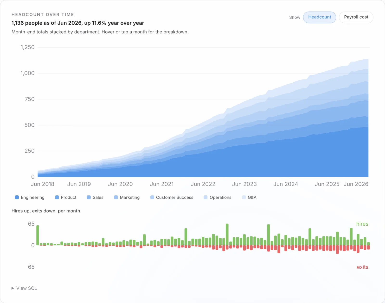
    headcount_cube.sql           #   month x dept x level x location
    tenure_turnover.sql
    representation.sql
    paygap_population.sql
    cost_per_hire.sql

Onboarding a client is rewriting the four or five staging models so their HRIS fields land in the canonical column names. The canonical models, the marts, the definitions, and the charts above them do not change. That is the difference between a bespoke project and a product you happen to deliver as a service.

Step 1: lock the grain, then reconcile to the source

The canonical event models are the contract everything else depends on, so they are tested before anything reads them. One row per person, one per comp event, one per req (grain). Termination date and type are null together or not at all (nulls). Every comp event resolves to a real person and the manager chain ends at exactly one CEO (referential integrity). And the number that earns trust in a client build: month-end headcount recomputed from the events ties to the active count in the source HRIS, every month. If it does not reconcile, the build fails and nothing downstream renders.

Step 2: the metric marts are the reusable core

Each insight is a GROUP BY mart with a stable output shape. The reusable engineering is mostly in the denominators, not the dashboards. Take annualized attrition: dividing exits by headcount is the common mistake, because a growing company is full of people who have not had time to leave. The right denominator is person-years of exposure, and that one pattern recycles across every turnover cut you will ever build (overall, by department, by tenure band):

-- Annualized voluntary attrition by tenure band.
-- The denominator is PERSON-YEARS of exposure, not headcount. A fast-
-- growing company is full of people who simply have not had time to
-- leave yet, and dividing by headcount would flatter every rate. Each
-- person contributes time to every band they actually passed through.
WITH bands(band, lo_day, hi_day) AS (
    VALUES ('0-6m', 0, 183), ('6-12m', 183, 365),
           ('12-18m', 365, 548), ('18-36m', 548, 1096), ('36m+', 1096, 99999)
),
exposure AS (                 -- person-years each band accrued
    SELECT b.band,
           sum(greatest(0, least(e.tenure_days, b.hi_day) - b.lo_day)) / 365.25
               AS person_years
    FROM employees e CROSS JOIN bands b
    GROUP BY b.band
),
exits AS (                    -- voluntary exits, placed in the band at exit
    SELECT b.band, count(*) AS vol_exits
    FROM employees e JOIN bands b
      ON e.tenure_days >= b.lo_day AND e.tenure_days < b.hi_day
    WHERE e.term_type = 'voluntary'
    GROUP BY b.band
)
SELECT b.band, round(x.vol_exits / e.person_years, 4) AS annualized_rate
FROM bands b JOIN exposure e USING (band) LEFT JOIN exits x USING (band)
ORDER BY b.lo_day;

The rest of the marts have the same shape and the same few lines. The headcount cube is month by department by level by location. The representation mart is a level-group cube with gender and ethnicity counts. The pay-gap population is one row per active employee with the controls attached. Cost-per-hire rolls the requisition components up by source and level. Because they are all pre-aggregated, the serving layer reads kilobytes whether the client has a thousand employees or a hundred thousand, and the same mart definition runs unchanged from one client to the next.

Step 3: define each metric once, in the semantic layer

"Voluntary turnover," "regretted exit," "fully loaded cost-per-hire," and the adjusted pay-gap model are defined once and consumed everywhere: by every chart, every filter, and any AI query pointed at the warehouse. Nobody re-types what counts as a regretted exit per report, so two dashboards can never quietly disagree. In the demo this shows up as a "View SQL" panel on every chart that regenerates as you filter: the number and the query that produced it are the same object, so they cannot drift. In a client deployment that panel is the governed semantic-layer query.

Step 4: build each chart as a component over its mart

Because the marts have a stable shape, a chart is a component that reads columns, not a client. The same scorecard renders this synthetic company or a real one, because both marts expose (month, dept, level, location, hc, hires, exits). In the demo every chart is hand-rolled SVG with no chart library, which is what lets each one ship its own View-SQL panel and recolor to a brand. In a client it is the same component in their BI tool or an embedded React app. The four chart families below are what the architecture produces, and each one carries a build decision worth naming.

Attrition is a tenure curve, not a number

The scorecard headline is 16.5% voluntary turnover, but the average hides the shape. Plot the mart from Step 2 and the risk is a cliff at 12 to 18 months, where people are past ramp and open to a recruiter:

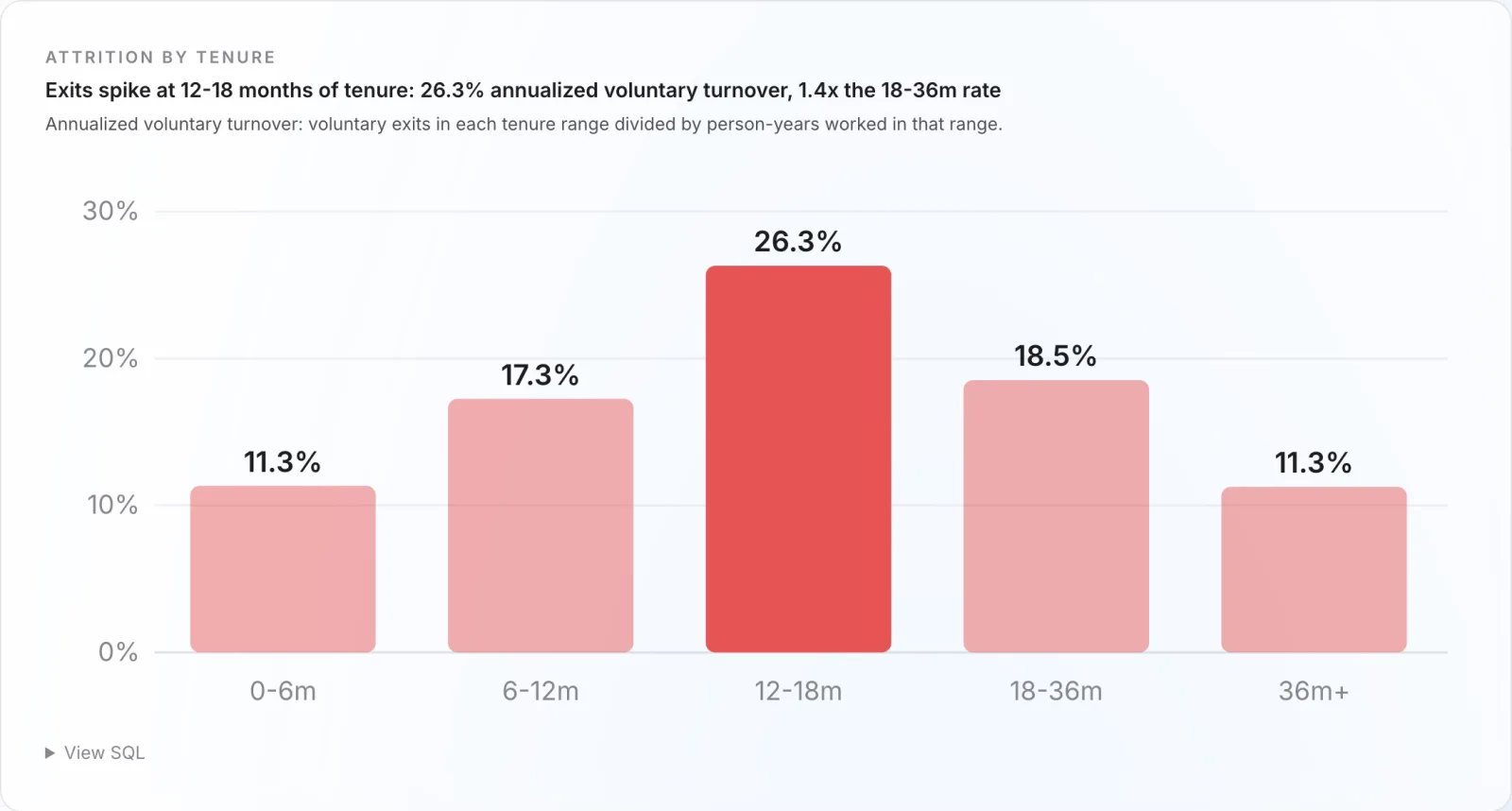
The same mart, cut by department, shows Sales bleeding 23.7% a year against Engineering's 12.1%, and 55% of voluntary exits are people the company rated a 4 or 5 and wanted to keep. One turnover percentage would have hidden all of it. The build decision: the chart is the tenure curve and the department split, never the single number.

Representation: build the de-confound in, or mislead by accident

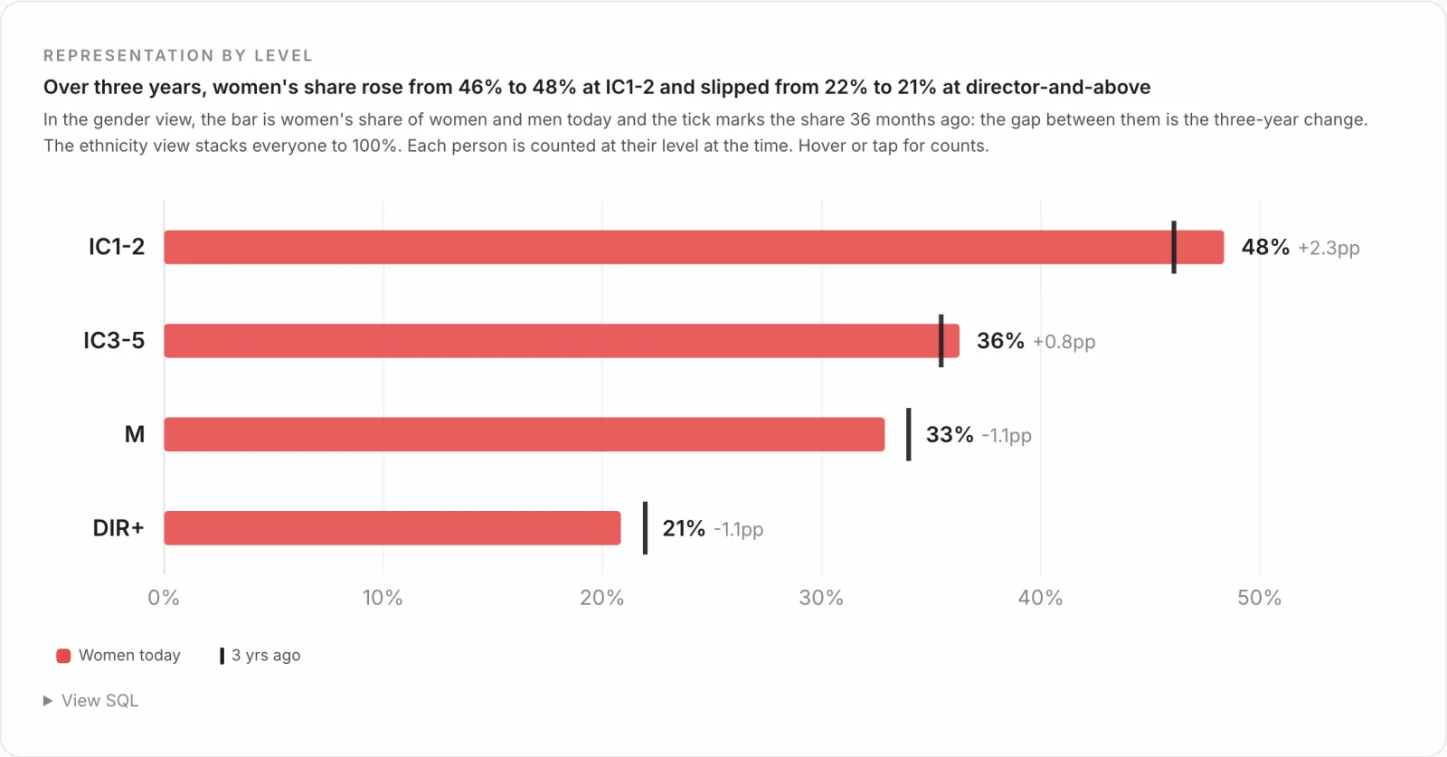
The gradient above, from 48% at the two junior levels to about a fifth at director and above, is where most representation dashboards stop. The dangerous follow-up is "do women get promoted more slowly," because the naive mart lies. Pool every promotion in Engineering and Sales and women look like they advance at least as fast as men. Hold hiring level constant and the gap reappears: women reach their next level at 0.93 times the rate of men. The pooled number was averaging across levels that promote at different speeds, which is Simpson's paradox, and the only honest version computes the within-level comparison. The reusable lesson is that the representation mart has to carry level so the chart can de-confound, because the convenient pooled cut is the one that quietly misleads a leadership team.

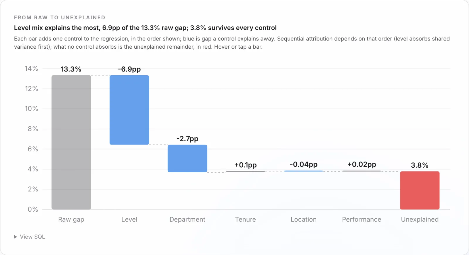
Pay equity: two models, because there are two questions

The unadjusted gap, every woman's median pay against every man's, is 13.6%. Hold level, department, location, tenure, and performance constant and it falls to 3.8%, and the confidence interval still excludes zero. Control for exact level and it drops again to about 1.2%. Three numbers, and the build job is to show all of them with the reason they differ, not to pick the flattering one.

It is the same definition, computed two ways:

-- Pay equity is one definition, computed two ways, on the same active
-- population (run as numpy least squares on log salary, women vs men).

-- Unadjusted: the raw gap, no controls. "Every woman vs every man."
--   log(salary) ~ female

-- Adjusted: controls join in a fixed order, so each step of the waterfall
-- is the gap after one more thing is held constant.
--   log(salary) ~ female + level_group + department + location
--                 + tenure + tenure^2 + performance_rating

-- The coefficient on 'female', as a percent, is the gap. Swap level_group
-- for exact level and it drops again: that last move IS the within-level
-- mix. Define it once here; every chart and every AI query reads it.

The module ends where an executive acts: a gender-blind remediation model flags everyone paid more than 10% below what their own level, department, and tenure predict, then prices the fix at 127 people and 2.31 million dollars a year, which is 1.63% of payroll. That is a budget line and a defensible method in one chart. On a client this model is the piece that needs the most governance: which controls, exact level or level group, signed off and versioned, so when legal asks why the number is 3.8% and not 13.6% the answer is on the page.

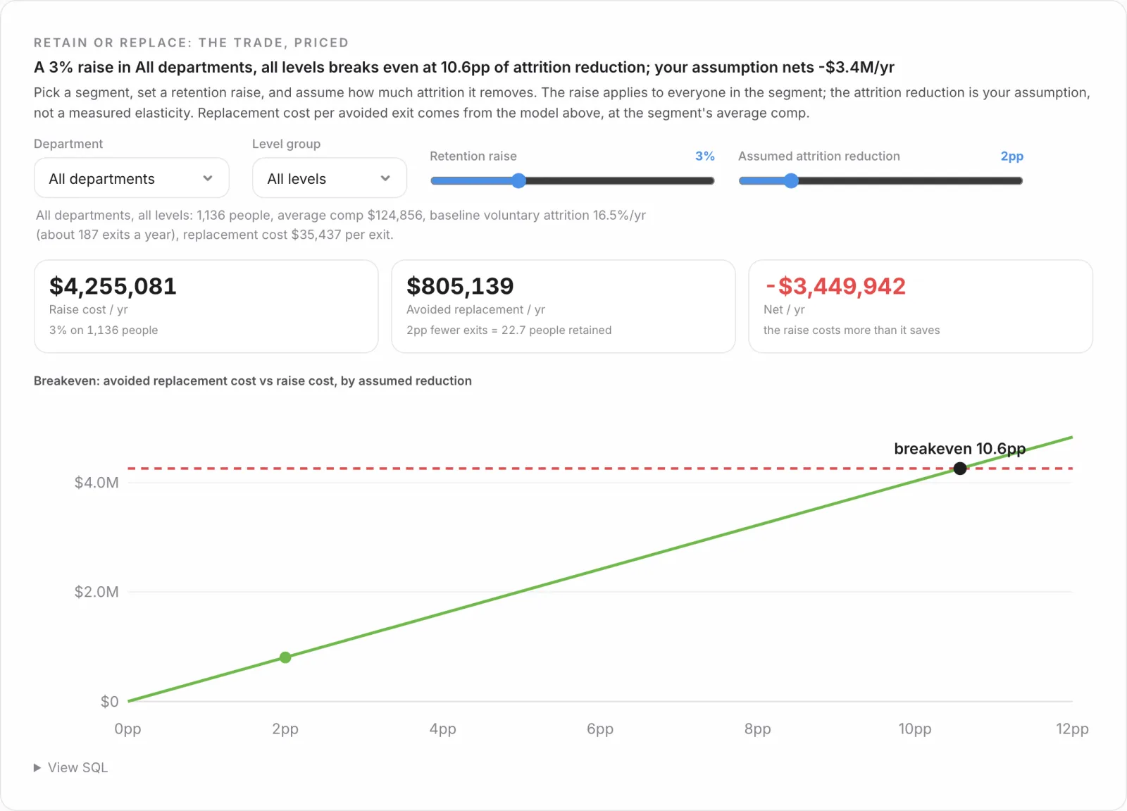
Retention economics: make the chart do the math

The last family turns retention into money. A hire is priced fully loaded, from about $4,500 for an inbound individual contributor to roughly $47,500 for an agency-sourced director, and replacing someone costs more than hiring them because you also eat the vacancy and the ramp. The payoff chart is a calculator: pick a department and level, set a retention raise and the attrition it would prevent, and it solves the break-even. A 3% raise across the whole company has to cut attrition by 10.6 points to pay for itself. Aimed at Engineering directors, where people are expensive to lose and slow to replace, the break-even drops to 5.3. The build decision is to ship the model, not a static number, so a manager finds the answer for their own team by moving a slider.

What recycles, and what does not

The honest accounting, because the pitch is the reusability. What recycles, unchanged, from one client to the next: the canonical event models, every metric mart, the semantic-layer definitions, the chart components, and the test suite. That is the bulk of the work and the bulk of the value, and it is already built.

What does not recycle: the staging models that map a specific HRIS onto the canonical tables, the access rules that match the client's org, and the calibration of the choices inside the definitions (the tenure bands, the suppression threshold, which controls go in the pay model). That is real work, but it is days, not quarters, because it is the only part you are doing from scratch. The four questions, the marts, and the charts came along for free.

The point is the time it gives back

The deliverable is not a dashboard. It is a tested dbt project, a governed semantic layer, and a set of chart components whose every number ties back to a query you can read. You own the repo, so the next question your CHRO asks is a new mart over models that already exist, not a new project and another month of plumbing.

That is the real return for a people analytics team. When the pipeline is reusable and the numbers tie out on their own, the work stops being about producing the chart and starts being about what to do with it: which 12-to-18-month cohort to invest in, which level to close the pay gap at first, where a retention raise actually pencils. The architecture is plumbing so that your week is not. That is how people analytics ends up improving how people experience the place and how efficiently it runs, instead of only reporting on it.

The suite is live here on synthetic data. The company is invented, but the framework is the one we would stand up in your warehouse: definitions in one place, and charts that read columns instead of clients. Point it at your data and you own a people analytics capability, not a dashboard subscription.

Josh